What are Neural Networks and how do they work?

To be precise, we are not dealing with an “invention” of the last few years here, but rather with a technology that was “invented” decades ago, but which only gained momentum about 15 years back due to technological innovations (computing power, availability of data, etc.). But we are not diving further into this topic: As there are so many misunderstandings and errors surrounding the topic of “neural networks”, we will address this issue in a separate article.

What are Neural Networks?

But what do we mean when we speak of “neural networks”? Technically, we talk about “artificial neural networks” (ANN), because “real” neural networks are only found in higher organisms, not in software or machines. In IT, however, the terms are interchangeable and usually describe artificial neural networks. Referring to “real” neural networks in living beings, one often speaks of biological neural networks for the sake of clarity.

Recently, Deep Learning replaced “neural networks” in common terminology. This is due to the fact that the latest and greatest results are only achieved if neural networks are built up from several layers, i.e. built “deep”. So, to be very precise, Deep Learning equals “machine learning with artificial neural networks built of several layers”. But even here the terms are used interchangeably: All interesting neural networks are “deep” anyway, so ANN and DL actually mean the same thing nowadays.

Artificial Neural networks – structure & function

There are many different types of neural networks (also called architectures). To solve a task, choosing the perfect and adequate approach is key. Often complex architectures consist of several simple networks, which are then combined in the right way. Unlike our brain, which can adapt dynamically to many tasks in a heartbeat, even the smallest of errors can cause a neural network to fail and not learn anything. If you choose the wrong architecture for a task, you usually have zero chance of getting good results.

Every architecture works differently, of course, but all neural networks have the same basic functionality, which is best explained with the most common neural network, the “fully connected neural network” or also “feed-forward neural network”, sometimes also somewhat inaccurately called multi-layer perceptron.

How a “Fully Connected Neural Network” works

Most other descriptions of neural networks would now begin with a biologically inaccurate description of neural networks and try to explain how ANNs work in computers. Unfortunately, this comparison is severely flawed and carries the great danger of creating a false perception of this technology. Therefore we leave the biological part out and start with a real ANN.

An ANN usually consists of several layers. A layer gets a (sometimes very large) sequence of numbers (vector) as input and creates a new sequence based only on this input. This new sequence of numbers can be shorter, longer or of the same size. Each layer usually carries out only very few arithmetic operations on the input numbers (e.g. a multiplication or addition).To get an idea of how a layer of a real artificial neural network works, let’s take a look at the Fully Connected Neural Network.

The three steps of the “Fully Connected Neural Network”

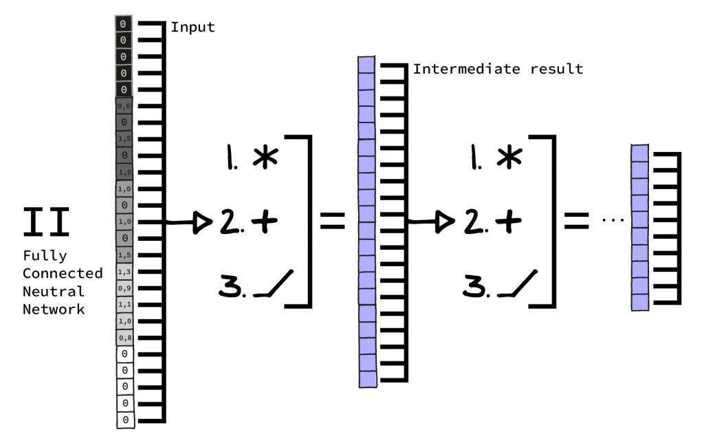
The Fully Connected Neural Network, for example, repeats the same three steps over and over:

1. multiplication with constants and addition of the results

2. addition of another set of constants

3. and a so-called activation function.

All three steps in a row add up to one “layer” of the neural network. In each layer a set of numbers is additionally stored. Frequently these numbers are called “weights”. Interestingly, the mathematics used by a neural network to calculate its results are extremely simple. Actually, even basic school knowledge is sufficient.

Let’s start with step 1: To calculate a single output value, each input value is multiplied by one of the numbers stored in the layer. The results of these multiplications are added up. The number of repetitions depends on the new values requested.

Let’s say we want to insert 768 values into a layer and get 512 results in return. In this case the process is repeated 512 times (once for each requested output) with all 768 values, each time with different numbers stored in the layer. So the network must hold 512*768=393,216 numbers in the layer for this step.

Step 2 is simple: To each result of the 1st step, another number stored in the neural network is added. In our example, this step requires 512 additional numbers in one layer.

Step 3 is even easier: The results from Step 2 are modified once more. This time we only check if the result is greater than zero, so we don’t need any stored numbers from the network. If the result is greater than zero, it is simply forwarded. If it is less than zero, it is replaced by zero. This is the activation function. Surprisingly simple for such an impressive name!

“Learning” through repetition and improvement

This three-step process of the Fully Connected Neural Network is repeated again and again for all layers of the ANN. But where do the numbers we multiply and add with come from?

Unlike the structure of the network (the amount of layers, the amount of input and output values), these are not defined by programming. Instead, random numbers are initially assigned. This means: a newly hatched neural network produces only nonsense from its input by wildly multiplying and adding random numbers.

Now the notorious “learning” comes into the equation. It works exactly as described in our blog article “The Basics of Machine Learning”. Whenever a neural network is supposed to learn something, it needs a series of inputs, accompanied by the requested result. The best test data set for neural networks here is the so-called MNIST data set. It consists of thousands of black and white images, showing handwritten single digits (0 to 9).

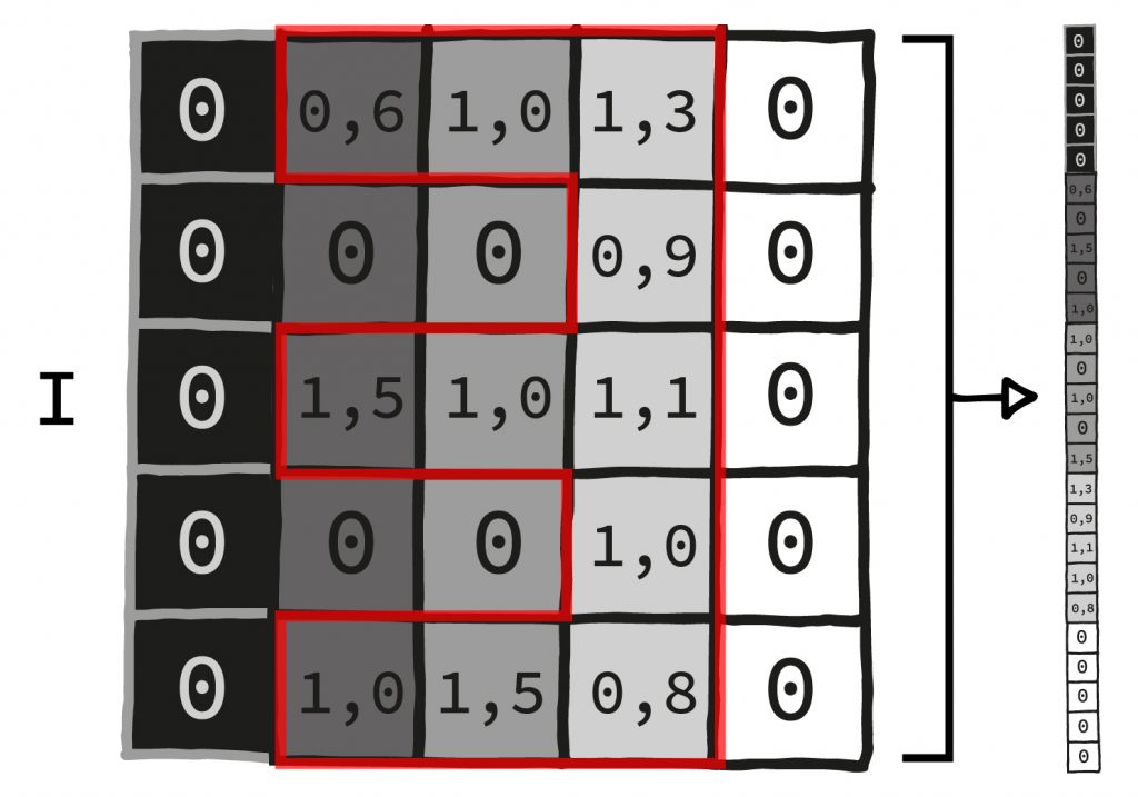
There is a solution for each pairing of picture and number. The pictures are  28 by 28 pixels in size. The neural network needs all pixels to calculate a result, so the first layer must be large enough for 28*28=768 entries.

Example of a Fully Connected Neural Network

If we want to “train” a Fully Connected Neural Network to assign the correct digit to an image (to “recognize” it, in human terms), we must first set it up in a reasonable way. If the set-up is correct, the neural network will gradually approach the correct classification of the images by means of the deviations, which are continually being corrected.

The Neural Network as Image Recognition: Setup

I. The input gets as many values as there are pixels in one of the MNIS digit images (28*28=784). So we insert all pixels into the neural net all at once.

II. Now we stack about five layers as described onto each other, i.e. we perform the process of multiplication and addition, addition and activation function for five times. The output of each layer is always smaller than its input. (This need not be the case with every neural network, but in this case it works well).

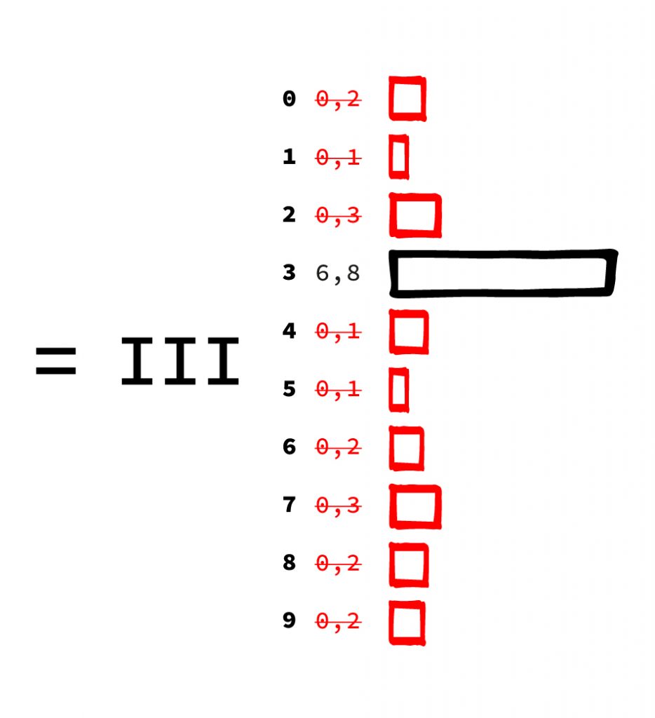
III. The last layer has 10 output values, one value for each possible digit to be recognized. Each value stands for how similar the net considers the input to a digit. Here you can see very nicely the “inaccurate” calculation of a neural network. It does not output a digit, but names the probability for each single result. Usually you simply choose the answer with the highest probability if you want a single answer.

Before we can train the network, the numbers used in each layer are filled with random numbers. This sounds pointless at first, but there is a very practical reason behind it: We don’t know how the network is supposed to solve the task – it is supposed to learn exactly that in the next phase. Since we ourselves have no idea, we randomly choose the starting point of the learning process by setting up random numbers.

Training and “backpropagation”

Now we have defined the structure of the network. You could even run the ANN on images now, but this would be quite useless: Due to the initialisation with random numbers the result is initially completely worthless. This changes with the next step – the training.

We use part of the MNIST images (about 90%) and feed them into the neural network, one at a time. Then we examine the outcome. This step is called Forward Pass, the images run straight through the net. We compare the ten output values with the actual result. For an image with a 3, the desired perfect result would be [0: 0%, 1: 0% , 2: 0%, 3: 100%, 4: 0%, 5: 0% … ]. We can now calculate by simple subtraction how wrong the neural network is for each percentage value. This numerical concept of “wrong” is the trick when training neural networks.

The calculated error is used to change the constants stored in the neural network with a special algorithm called “backpropagation” in tiny steps. To do so, the error is “split” over all layers and all constants are adjusted a little bit upwards or downwards. The algorithm determines mathematically which part of the network has caused the most severe error and, weighted accordingly, “compensates” by adjusting the constants. This is the so-called backward pass, as the error runs backwards (from output to input) through the network.

The next time, the network will be slightly less off-target and the process is repeated. This has to be done for quite a while. For simple problems like the MNIST images, a few tens or hundreds of thousands cycles are needed. For severe problems like the detection of pedestrians for a self driving car, you may have to do it a few billion times. Here you can see a clear difference to our brain: humans can learn a task using far, far fewer examples.

Review of the training using the test data

If the error in training is small enough, you stop training. Then the last 10% of the data (test data) that we have not used for training comes into play. The network has never seen these before and therefore was not able to “learn them by heart”. That way we check if the network can really recognize numbers. If the network is able to deliver the correct answer to an acceptable amount of images it has never “seen” before, we have successfully trained our first neural network.

If it is thoroughly wrong on this so-called test set, although the error during training was nice and low, we have so-called “overfitting”. The net did not learn to abstract, but only learned the training pictures by heart. We made a mistake somewhere and have to start all over again.