The basics of Machine Learning

Only this enables the computer to correctly access the “learned” answers (be it in the form of a decision tree or a table) and lets the program solve the problem in a comprehensible way. However, this also means that an algorithm can only provide the solution to a very specific problem. The moment the problem changes, the algorithm must be modified (or rewritten).

This is exactly where machine learning really comes in. The aim of machine learning is to allow the computer to formulate and solve the problem - i.e. to enable it to take over the “unpleasant part” of adjustment and fine-tuning itself. To do this, a machine learning program is equipped with two different algorithms, a learning algorithm and an inference algorithm. Equipped with those, the same (or very similar) program can ideally solve many different problems, while applying the same method - instead of programming everything from scratch.

On a side note, the term “learning” should be used with caution: People tend to anthropomorphise, i.e. we like to attribute human qualities to inanimate objects: Everyone has probably scolded their computer at one point or another - knowing fully well that it neither hears nor understands what is said. If we now say that computers (or rather: algorithms) “learn”, then there is a great danger of us understanding this learning process as analogous to the human learning process. But as we’ll soon discover, machines “learn” quite differently. That’s why most ML developers prefer to talk about “training” their algorithms.

The most important ML terms, explained simply

The best way to understand how ML works? Going over an example step by step. But before we plunge right into it, we need some essential ML vocabulary first:

• Algorithm: An algorithm is a fixed, finite sequence of instructions, used to perform a particular calculation. Each computer program consists of a number of different algorithms. An algorithm can be very simple (“Find the smallest number in this list of numbers”) or very complex (“Train this neural network”). Most ML methods work with two algorithms: The so-called training algorithm trains the program based on the available data, the so-called inference algorithm applies the gained " findings " and delivers results.
• Parameter: A value that is learnt during the training of a machine learning program. Based on existing parameters, the training algorithm “trains” and tries to continuously improve the parameters. The inferencel algorithm uses the parameters to calculate results.
• Model: A trained machine learning method. A model is essentially a (sometimes very large) set of parameters and instructions on how to use them - a ready-to-run ML procedure and the result of the training process. The training algorithm generates the model, the inference algorithm uses it to perform a task.
• Inference: Running a model using a second algorithm. This algorithm uses the model to create a prediction based on an input, classify an input or create some interesting value based on an input. Hence the term “inference algorithm” or “prediction algorithm”. Inference is a technical term for “execute the ML model and output a result”.

As we see, Machine learning use the combination of a training algorithm and a prediction (or inference) algorithm. The training algorithm uses data to gradually determine parameters. The set of all learned parameters is called a model, basically a “set of rules” established by the algorithm, applicable even to unknown data. The inference algorithm then uses the model and applies it to any given data. Finally it delivers the desired results.

Procedure of a Machine Learning Training

Equipped with the right vocabulary, we can take a closer look at the execution of a machine learning project:

1. We select the machine learning method for which we want to train a model. The choice will depend on the problem to be solved, the available data, the experience and also on gut feeling.
2. Then we divide the available data into two parts: The training data and the test data. We apply our training data and thus obtain our model. The model is checked on the unknown test data. It is most important that the test data aren’t used during the training phase under any circumstances. The reason is obvious: Computers are great at learning by heart. Complex models like neural networks can actually start to memorize by themselves. The following results might be quite remarkable. There’s only one flaw: They’re not based on a model formulated by the program, but on “memorized” data. This effect is called “overfitting”. However, the test data are supposed to simulate the “unknown” during quality control and to check whether the model has really “learned” something. A good model achieves about the same error rate on the test data as on the training data without ever having seen it before.
3. We use the training data to develop the model with the learning algorithm. The more data we have, the “stronger” the model becomes. Using up all available data for the training algorithm is called an “epoch”.
4. In order to test it, the trained model is used on the test data unknown to it and makes predictions. If we did everything right, the predictions on unknown data should be as good as on the training data - the model can generalize and solve the problem. Now it is ready for practical use.

A Machine Learning project - step by step

Now that we have gone through the individual steps theoretically, we should put them to use on a specific example. Doing this we also want to introduce the most important ML algorithm - Linear Regression.

The most important ML algorithm: Linear Regression

Applying the steps we just established, we first have to decide on the most suitable algorithm for the particular problem. Selecting an algorithm is the first step in our Machine Learning process. We described the algorithm as a guideline,  specifying how the computer should handle certain data. An especially important algorithm in Machine Learning is the so-called Linear Regression. All the basic components of ML may be found here. Even though other methods are far more complicated, they all work according to the same principle. You might also know linear regression from spreadsheets by the term “trend line”.

So what does the impressive term “Linear Regression” actually mean? A regression is a problem that - based on several entered variables or values - “spits out” one or more numerical values. An example of a regression, for example, is a tax return: After entering a series of values, the end result is the tax to be paid. Or the calculation of a braking distance: The speed is entered, the expected braking distance is given.

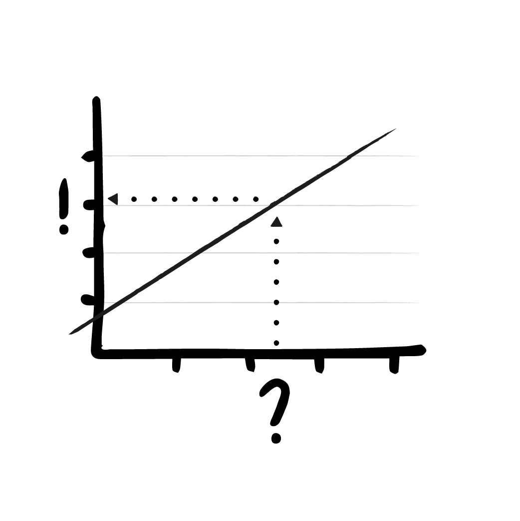
Not wanting to complicate things further (and in order to make our example easier to display), we will limit ourselves here to the simplest form of linear regression, where there’s only one value entered and one value output. A certain value on the x-axis results in a corresponding value on the y-axis. The values can be displayed as points in a coordinate system.

This simple procedure has merely two parameters: On the one hand, there is the slope and the offset of the line. These two values are gradually adjusted by the training algorithm.

In this case the inference algorithm is very simple as well: Based on the input (the x-value) the output is calculated, by looking at the corresponding y-value of the line at this point.

Putting ML into praxis - Linear Regression, step by step

Lying on a meadow, looking into the night sky, listening to the chirping of the crickets… we ask ourselves: How often per second do the crickets chirp? We assume that crickets (as insects) like it warm and that the intensity of chirping depends on the temperature. We want to calculate this for all temperatures, but we cannot control the weather to get the data. Besides, we obviously don’t want to lie around night after night with a microphone and a thermometer.

Step 1 - Choosing the right ML procedure

So we have two readings that seem to be linearly dependent on each other. The warmer it gets, the more intense the chirping of the crickets seems to be: Before our inner eye we see a linearly ascending line - and decide to use linear regression as the probably best method!

Step 2 - Training and test data for the training algorithm

In order to “learn” something, our training algorithm needs at least some data. So we take heart, pack our measuring equipment, visit the meadow and collect the training and test data for our ML method. (Or we simply download the data here). Before we “feed” the model with the first batch of data, it’s parameters are set to a value first. These initial values for the parameters of the model are either random numbers or zeros (depending on the parameters and the ML method). Without having learned anything, the model can at least spit out values without crashing. Though, of course, these values are totally wrong.

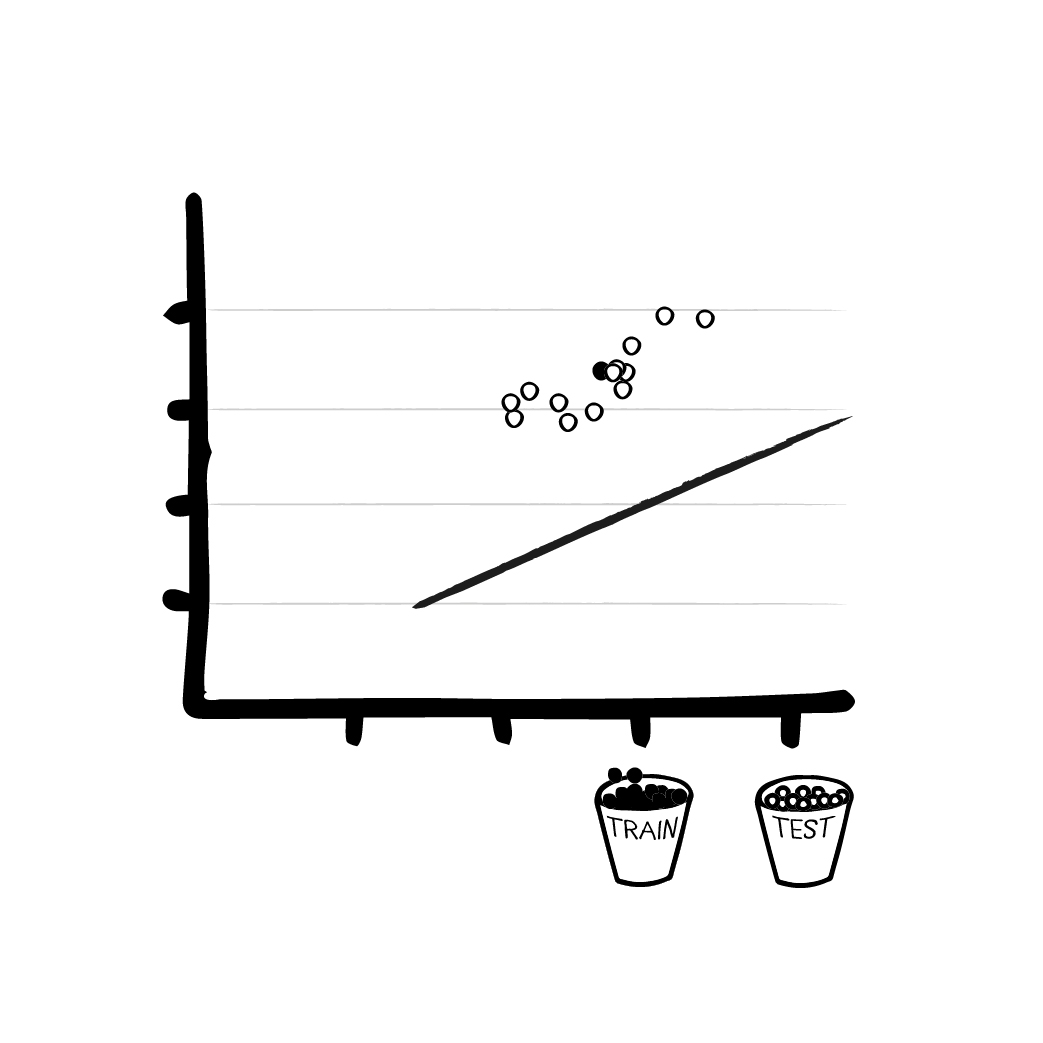
Step 3 - Training the ML model

To start the actual training session, we enter a set of training data into the model and calculate the (probably entirely wrong) results. Because of the random initial values, the model first guesses the results at random. The random values in this initial formula cause the model to spit out meaningless numbers. But at least we have a result, even if it is wrong.

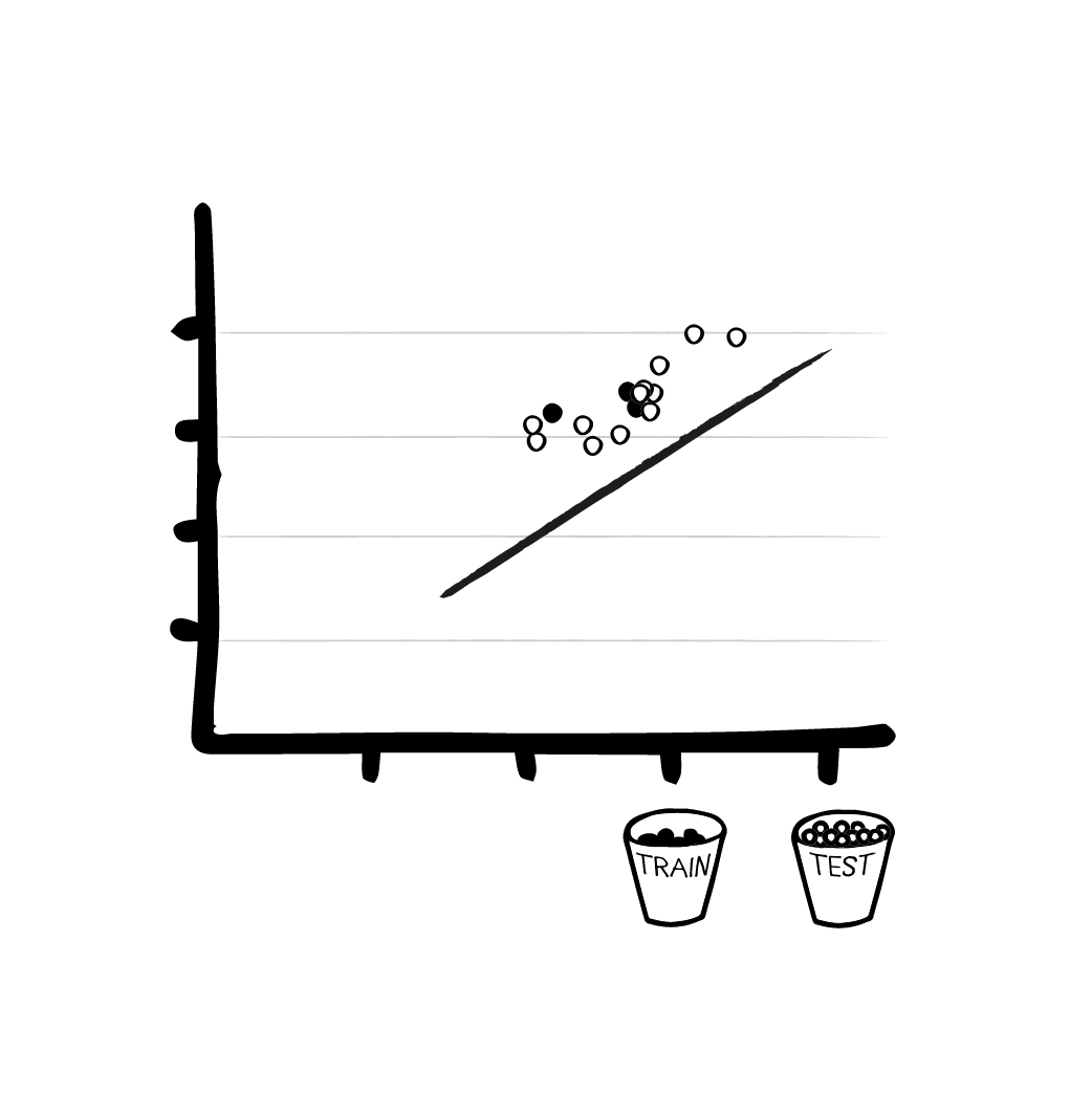
Now we can use a trick: We calculate the error. The larger the amount of test data, the clearer the picture of the errors and deviations becomes. The inference algorithm calculates the current prediction of the model. The training algorithm compares the prediction with the actual correct result in the training data and computes how much they differ. This deviation is used to adjust the parameters in order to improve the next prediction. The algorithm gradually improves our linear function, monitors the deviations and “registers” whether they are increasing or decreasing, depending on how the parameters are adjusted. In short, it states how we need to change our model to better match the data.

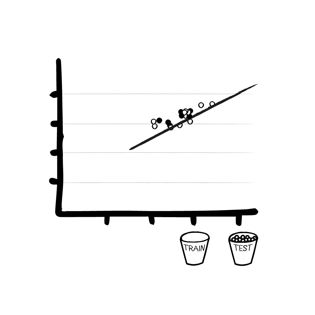
Step 4 - Checking against the test data

Without immersing ourselves too deeply in mathematics, let us put it this way: With the right formulas, the training data and the initial (wrong) output of the model, the algorithm can optimize the parameters and thus get a better solution next time. Using linear regression, as we did in our case, this is done by moving the line closer to the training points.

1. We take a batch of training data, calculate the result.
2. We calculate the error and observe how much the result is wrong (e.g. by simply computing the difference to the desired result).
3. Based on the error and clever mathematics (mostly derivatives) we calculate how we have to change the model to minimize the error.
4. When we are satisfied with the result, we stop - if not, we go back to 1. and we repeat all the steps with another part of the training data.

So what would happen if we used up all the training data and are still not happy with the result? Easy: We initiate a new epoch (see above) after putting the data in a new random order. Ideally there is so much data as to never reach the end of an epoch. In practice, however, data is often used several times, i.e. the model is trained over several epochs. It’s somewhat similar to a human learning a foreign language: We often have to go through the new vocabulary several times (and if possible in alternating order) until we have learned it.

Linear regression and ML dealing with “high-dimensional input”

Maybe people might think: “But that’s cheating! Drawing a line through a few points isn’t AI!” However, you have to keep in mind that the same method works not only with a simple one-dimensional function, i.e. one input and output value, but also with so-called “high-dimensional input”.

This rather pompous term merely implies that one has several input variables. It is therefore more related to a tax return than to science fiction: Every tax return has a multidimensional input (wage, independent income, number of children, …). A letter is also addressed by multidimensional entries: Name, surname, company, address supplement, street, house number, postal code, city, country - here we are at a 9-dimensional input!

Our cricket example had only one input and one output value, so that we could display the data sets two-dimensionally as a graph. But the same mathematics that can be employed to train a simple linear regression with one input and output will also work for any number of dimensions. Referring to the underlying mathematics, it is still called “linear” - even though the drawing of the model isn’t and can’t even be depicted graphically as a line - if at all.

ML in practice: As simple as possible, as complicated as necessary

We conclude: With proper pre-processing, a Linear Regression can be amazingly performant. That’s why this simple algorithm still has so much practical relevance. On the one hand as a element of more complex systems - as we will see later, no Neural Network can do without Linear Regression. On the other hand, simple methods often perform better than complex ones, when it comes to Machine Learning. The quality of the result usually depends less on the method, but rather on the training data. Also, the performance gained by a complex procedure can be so low that the increased effort (computing time, storage space, programming effort, fine-tuning, …) for the complex procedure is not really worthwhile.

In any case, linear methods are always well suited to define a “baseline”: What can be achieved with minimal effort using existing data? Many projects start with a linear method as a baseline in order to better estimate the quality of later results.

Of course, there are a lot of things that linear regression cannot do - otherwise there would be no need for Deep Learning or Neural Networks. But as with the methods of Symbolic AI we have presented before, the following holds true: As simple as possible, as complicated as necessary. In a real project, the aim is to achieve the best possible result while wasting as few resources as possible.

So what happens next? We will look further at Machine Learning and discuss how to further categorize ML procedures. We will also consider their advantages and disadvantages.